If you want better schedule forecasts on Azure, the answer is simple: build one clean activity history, train with time-based data splits, score in batch by default, report in Power BI, and lock the whole flow down with access, lineage, and audit rules.
I’d boil the full guide down to this: forecasting activity duration works when data, models, reporting, and governance are tied together from day one. The article shows how to move raw schedule files and field data into ADLS Gen2, shape an activity-level feature table, train models like XGBoost or LightGBM, publish forecast results to Power BI, and track each prediction back to its source. It also makes one point very clear: if even one part is weak, forecast quality drops fast.
Here’s the short version of what matters most:
- Start with one forecast unit: one activity, at one point in time
- Use Azure storage by purpose: ADLS Gen2 for raw and staged data, Azure SQL Database for smaller curated sets, Synapse for very large history
- Train with time-based splits: not random splits, so you don’t leak future data
- Track core metrics: MAE, RMSE, MAPE, plus forecast hit rates like ±10% or ±2 days
- Use batch scoring first: it usually costs less because compute runs only when jobs run
- Publish governed outputs: scored durations, confidence ranges, slippage, and overrun probability in Power BI
- Control access and traceability: Entra ID groups, private endpoints, Key Vault, Purview, model registry, and approval logs
A few points stand out. The guide separates storage choices by scale, keeps Microsoft 365 inputs limited to approved aggregate signals, and pushes teams toward three environments: dev, staging, and production. It also treats model review like a release process, with checks for data quality, error levels, security, and business sign-off before a model goes live.
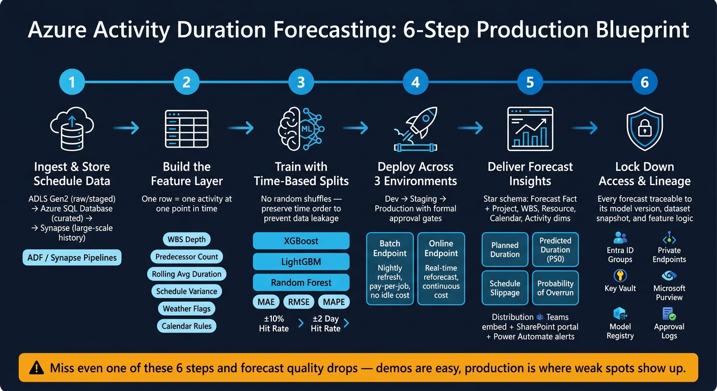
Azure Activity Duration Forecasting: 6-Step Production Blueprint
Quick Comparison
| Area | Main Recommendation | Best Default |
|---|---|---|
| Data storage | Split raw, curated, and archive layers | ADLS Gen2 + Azure SQL Database |
| Model family | Start with tree-based models | XGBoost / LightGBM |
| Train/test method | Keep time order intact | Time-based split |
| Inference | Use nightly refresh unless same-day reforecast is needed | Batch endpoint |
| Reporting | Serve scored forecast tables to planners and leaders | Power BI Import mode |
| Governance | Separate environments and log each model version | Dev / staging / production |
In short, I see this guide as a production blueprint, not just a modeling walkthrough. It’s about making sure forecast outputs are usable, trusted, and easy to trace when schedule decisions are on the line.
Design the Azure Data Flow for Activity History and Forecast Inputs
Start with a governed path from source schedules and field logs into Azure. That gives you one place to standardize the data before training.
Ingest and store schedule data in Azure
Land raw files in ADLS Gen2 using source-based and date-based folders. From there, move the data through staged and curated layers with Azure Data Factory or Synapse Pipelines.
Store Microsoft Project and Primavera P6 files in SharePoint or OneDrive, then ingest them on a set schedule with ADF. Connect ERP and CMMS systems through REST, SQL, or ODBC, and use watermark-based incremental loads. Keep each raw file unchanged, along with JSON metadata for timestamp, source path, checksum, and pipeline run ID.
Curated tables like FactActivityHistory, DimProject, DimResource, and DimCalendar should live in Azure SQL Database for smaller datasets, or in Azure Synapse Analytics dedicated SQL pools when history covers millions of activities across many years. Add lineage keys such as SourceFileId and IngestionRunId to every table so downstream models and reports can trace each record back to its origin.
Once the raw schedules are curated, turn them into one activity-level feature table for training.
Build the feature layer for duration prediction
Build FeatureActivityDuration from schedule structure, past performance, resource mix, calendar rules, and external signals. Each row should represent one activity instance at one point in time. That gives the model a stable unit of prediction.
Key inputs include:
- WBS hierarchy depth
- Predecessor and successor counts
- Rolling actual-duration averages for similar activities
- Schedule variance trends
- Working hours per day
- U.S. holidays
- Non-working days within the planned window
Weather data also matters. Temperature, precipitation, and extreme-weather flags aligned to the activity window help the model account for seasonal effects, like slower outdoor work during winter.
Compare storage and Microsoft 365 integration options
The right storage layer depends on data volume, query patterns, and governance needs. Here’s how the main Azure options fit into a forecasting setup.
| Storage Option | Primary Use | Governance | Implementation Effort | Best Fit |
|---|---|---|---|---|
| Azure Blob Storage | Raw file landing (MPP, XER, CSV), archival | Basic RBAC | Low | Simple file storage, backups |
| Azure Data Lake Storage Gen2 | Raw and staged analytics data, feature engineering | Fine-grained ACLs, hierarchical namespace | Moderate | Core storage for forecasting pipelines |
| Azure SQL Database | Curated tables, Power BI reporting | Mature (RBAC, row-level security, auditing) | Moderate | Small to medium datasets, simpler architectures |
| Azure Synapse Analytics | High-volume historical data, large-scale ML workloads | Enterprise data warehouse standards | Higher | Millions of activity records across many projects |
In practice, most production setups use ADLS Gen2 for raw data and feature storage, Azure SQL or Synapse for curated analytics tables, and Blob Storage for low-cost archival.
Schedule history is the starting point. Microsoft 365 should add context only when that context improves prediction and can be governed cleanly.
| M365 Access Path | Implementation Effort | Governance | Best Use |
|---|---|---|---|
| Microsoft Graph API | Moderate to high (API integration, token management) | Strong (Azure AD app registrations, scoped permissions, audit logs) | Automated, recurring signals like aggregated calendar load or document activity |
| File-based exports (SharePoint/OneDrive) | Low to moderate (built-in ADF connectors) | Good (SharePoint/OneDrive permissions, document library policies) | Batch schedule data - weekly Project or P6 file updates |
| Controlled manual uploads | Low (upload workflow via SharePoint library or Power Apps) | Moderate to strong (depends on workflow enforcement) | Ad-hoc or low-frequency inputs; higher risk of governance gaps without strict controls |
Microsoft 365 signals should be used only when they add clear model value and can be handled in the right way. Aggregated project-level metrics, such as document revision counts per week or average meeting hours for key roles, are fair game. Individual-level behavioral data is not. Use Azure AD app permissions to read metadata and counts, not message content.
With curated history and feature tables in place, the next step is model training and evaluation on Azure.
Train, Deploy, and Monitor Forecasting Models on Azure
Once you have the curated feature table, the next step is to turn it into a time-aware training pipeline. Keep the workflow modular: data loading, feature engineering, training, evaluation, and registration should each run as separate components in Azure Machine Learning or Databricks. That setup makes reruns much easier, keeps the process auditable, and makes handoff to another team far less messy.
Set up model training and evaluation
Split the duration target into train, validation, and test sets with a time-based split. Don’t use a random shuffle. If you do, future schedule data can slip into training, which makes metrics look better than they are and usually leads to weaker production results.
Log every run in Azure Machine Learning experiment tracking or MLflow. That includes the dataset version, feature set, hyperparameters, environment details, and evaluation results. Only register models that pass your preset thresholds. Also store the preprocessing pipeline with the model so training and inference use the same steps.
For evaluation, start with MAE, RMSE, and MAPE. Those are your baseline metrics. But don’t stop at one top-line number. Break results out by activity class, criticality, and duration bucket. A model can post an acceptable overall MAE and still miss badly on critical-path activities. It also helps to measure the share of forecasts that land within schedule tolerance, such as ±10% or ±2 days. That connects model choice to what planners can actually live with.
Gradient boosting methods - XGBoost and LightGBM - are strong defaults for tabular schedule data. They work well with mixed feature types, nonlinear relationships, and missing values without a lot of preprocessing. Start there. Bring in more complex models only if that simpler baseline can’t hit your error target.
Implement MLOps across dev, staging, and production
Use three separate environments: dev, staging, and production. Each one should have its own data, compute, and deployment controls. In dev, data scientists test features and model ideas. In staging, the full pipeline runs on a production-like dataset and checks quality, latency, and integration behavior. Production should only receive model versions that clear formal approval gates.
Automated CI/CD should handle code tests, infrastructure setup, pipeline runs, and endpoint deployment. Human approval gates are best saved for high-risk releases or model changes tied to critical schedules. Azure’s MLOps v2 guidance explicitly defines a staging phase where candidate models are retrained on representative production data, subjected to data quality checks, model bias checks, and performance tests, and only then promoted with human approval. [1]
For most forecasting use cases, batch scoring is the right default. Nightly jobs can refresh the forecast table before morning planning meetings. Azure ML batch endpoints only provision compute when a job runs, so there’s no charge while the endpoint sits idle if minimum instances are set to 0. [2][3][4] Online endpoints fit cases where planners need an immediate reforecast after entering a new activity, delay, or resource change during the day. A practical setup is simple: use batch scoring for the standard daily forecast table, and use online scoring for exception handling or interactive what-if analysis.
Store every approved model with its data version, code version, and training run. That way, when schedules shift, you can trace what changed and why.
After deployment, monitor data drift, feature distribution shifts, prediction error against later actuals, latency, and error rates. Segment results by project, region, trade, and critical-path status. Hidden model decay in one activity class may never show up in the aggregate view. Set retraining triggers ahead of time, such as a sustained increase in MAE or a material shift in input distributions, so the team can act before forecast quality starts hurting schedule decisions.
Compare model families and inference options
The best model family depends on how stable the schedule patterns are, how much critical-path errors matter, and how often forecasts need to refresh. Keep it simple: use the least complex model that meets your error and latency targets.
| Model Family | Best Fit for Duration Forecasting |
|---|---|
| XGBoost / LightGBM | Strong default for tabular schedule data; handles nonlinear relationships, mixed feature types, and missingness well |
| Random Forest | Useful baseline when robustness and stability matter |
| Support Vector Regression | Can work on smaller, cleaner datasets but tends to scale less well |
| Ensemble approaches | Helpful when activity types have different duration drivers |
| LSTM / CNN–BiLSTM | Better for repeated activities with stable temporal patterns, but requires more data and tuning |
The same tradeoff applies to inference. Batch is simpler and usually cheaper. Online is faster, but it comes with more overhead and continuous runtime cost.
| Inference Pattern | Latency | Complexity | Monitoring Needs | Cost Profile |
|---|---|---|---|---|
| Batch (Azure ML batch endpoint) | Minutes to hours | Low to moderate | Drift and error checks on each run | Pay-per-job; no idle cost when minimum instances = 0 |
| Online (Azure ML managed endpoint) | Seconds | Moderate to high | Real-time latency, error rate, and drift monitoring | Per-minute instance cost; runs continuously |
Online endpoints add extra operational work and steady cost, so they make the most sense for actual real-time reforecasting. These forecast outputs then feed the reporting layer in Power BI.
Deliver Forecast Insights in Power BI and Microsoft 365
Build the reporting layer for schedule risk
With scored durations stored in Azure, the next move is to turn that output into governed, report-ready tables.
When Azure ML batch scoring writes predicted durations and confidence intervals back to Azure SQL or a lakehouse table, Power BI can connect straight to those scored results. Set up a star schema with a forecast fact table tied to project, WBS, resource, calendar, and activity dimensions. Each row should represent one activity at one snapshot date. That gives you a steady time-based grain for rollups and trend analysis.
Expose four core measures:
- Planned Duration
- Predicted Duration (P50)
- Schedule Slippage
- Probability of Overrun
Then add baseline, actual, confidence interval, variance, risk score, and finish-date impact as support fields. Hide surrogate keys and other technical columns from report authors. Put reusable measures in a named measure table so every report pulls from the same definitions. Treat the governed Power BI semantic model as a certified data product with clear ownership and a refresh SLA.
Keep the reporting setup simple: one executive page for portfolio KPIs, and one drill-through page for drivers, baseline vs. predicted duration, and historical performance.
Design visuals and distribution workflows
Once the model is ready, shift focus to how planners will use the forecast and what they need to do next.
Use visuals that make exception, exposure, and next action easy to spot. A risk matrix, ranked exception table, waterfall, and baseline-vs.-predicted scatter plot cover the main use cases. Conditional formatting and threshold bands help operations teams spot low-float activities and likely critical-path impact fast.
For distribution, embed the report in Teams for shared review and use SharePoint as a controlled project portal. Power BI data-driven alerts can trigger Teams posts, emails, or Power Automate actions when slippage or uncertainty passes a set threshold. Route exceptions straight to named owners with a link to the exact report page they need. Threshold rules can also be parameterized by project type or contract risk profile.
Once people can see and share forecast insights, the next job is to lock down access, lineage, and auditability in the governance layer.
Choose the right Power BI connectivity pattern
Pick the connectivity pattern based on freshness and scale. Import mode is usually the best default for forecast reporting because visuals load fast and DAX modeling works well, as long as scheduled refreshes happen often enough. DirectQuery makes sense when you need near-real-time access to live schedule transactions or when the source is too large to import. Composite models work well when part of the model needs in-memory speed and another part must stay live, like imported forecast snapshots paired with DirectQuery access to current schedule transactions.
| Connectivity Pattern | Performance | Data Freshness | Best For | Key Constraint |
|---|---|---|---|---|
| Import | Fastest | Refresh-dependent | Most forecast reporting; rich DAX modeling | Dataset size limits; not real-time |
| DirectQuery | Slower; depends on source performance | Near real-time | Large datasets; live schedule transactions | Query load on source; limited modeling flexibility |
| Composite | Mixed; imported dimensions are fast | Mixed | Scenarios needing both speed and freshness | Higher design complexity; governance overhead |
On large forecast fact tables, enable incremental refresh so you don’t keep reloading unchanged historical snapshots. Apply row-level security on dimensions, not the fact table.
Governance, Security, and Production Readiness
Apply governance across data, models, and access
Production readiness comes down to control. You need clear rules for access, movement between environments, and what happens when something fails.
Start with environment segregation. Keep dev, staging, and production in separate Azure subscriptions or resource groups. As workloads move closer to production, tighten access. Use Azure Entra ID groups to manage permissions across the data, model, and reporting layers. Those groups should map to business roles, so access matches what people actually do on the job, not what happens to be convenient.
For networking, use private endpoints and managed identities instead of connection strings or long-lived credentials. Store secrets in Azure Key Vault. Limit storage accounts and ML endpoints to approved networks only. Encrypt data at rest with platform-managed or customer-managed keys, and enforce TLS for all data in transit.
Use Microsoft Purview to manage lineage and classification. Register schedule history tables, engineered feature sets, and scored output tables as governed assets. Purview’s glossary and classification tools help document what each asset contains, who owns it, and how it moves through the pipeline.
Apply the same controls to Microsoft 365 inputs before they reach the feature layer. If Microsoft 365-derived signals, such as Planner task data or SharePoint schedule exports, feed the feature layer, treat them as governed inputs too. That means documented retention rules and approval rules. Only ingest the smallest usable subset, and record that scope in your governance record.
Once access and environments are under control, the next step is simple: every prediction should be traceable back to where it came from.
Make forecast outputs auditable and traceable
Every forecast shown in Power BI should tie back to its model version, dataset snapshot, and feature logic. Azure ML’s experiment tracking and model registry record training runs with dataset versions, code versions, hyperparameters, evaluation metrics, deployment artifacts, and inference timestamps. Each production deployment should also link to a registered model version with a documented approval record.
Before a new model version reaches production, it should pass:
- offline evaluation
- feature review
- security review
- business sign-off
- deployment approval
Store monitoring outputs, approvals, and retraining decisions in the audit trail. If someone asks, “Why did this forecast look different last month?” you should be able to answer without digging through scattered logs and emails.
Apply Responsible AI guardrails before go-live. Use the Azure Responsible AI Dashboard to check for bias across project types, teams, or schedule patterns. Keep a model card that explains intended use, training data boundaries, known failure modes, and the conditions where the forecast is unreliable. Report consumers also need a plain-English warning: predicted durations are probabilistic estimates, not guaranteed commitments.
With lineage, approvals, and monitoring in place, the system is ready to operate in production.
Conclusion: The minimum production blueprint
A production-ready activity duration forecasting system on Azure depends on six connected pieces.
- A clearly defined forecasting scope tied to specific schedule decisions
- A governed Azure data flow that ingests, cleans, and versions schedule history in a reliable way
- A stable feature layer built on schedule attributes that predict duration
- An MLOps pipeline that trains, evaluates, and promotes model versions through controlled release gates
- A Power BI reporting layer that delivers scored forecasts to the right people through Microsoft 365 with governed access controls
- Governance controls - RBAC, lineage, drift monitoring, and audit trails - enforced before the system supports live operational decisions
Miss even one of those six pieces and the system may still look fine in a demo. But demos are easy. Production is where weak spots show up fast.
Teams that need delivery support can use Ryshe for senior-led AI, data, automation, and governance delivery.
FAQs
How much historical activity data do I need to start?
There’s no fixed minimum. How much historical data you need comes down to your operating context and how complex the work is that you’re trying to model.
Start with an audit of the data you already have, like ERP transactions, production logs, and activity records. A practical way to begin is with one high-value use case. Then, as confidence grows and data coverage improves, you can expand from there.
When should I use batch scoring instead of online scoring?
Use batch scoring when you need to handle large amounts of data on a set schedule, not return results right away. It works well for jobs like daily or weekly forecasts, scheduled reports, or batches of past maintenance logs.
It can also cut compute spend by avoiding the overhead that comes with always-on real-time systems. Pick it when the goal is steady, dependable insights delivered at planned intervals.
How do I keep forecast outputs auditable in production?
Use a governance and monitoring framework built around transparency and traceability.
In Microsoft Fabric, set up data lineage so each forecast can be traced back to its source. For system activity and usage, use Application Insights to keep audit trails in place.
You should also add:
- Automated data quality checks
- Error handling
- A central data catalog that shows dataset ownership and purpose
- Clear metadata and source documentation for every output
That way, teams can see where data came from, who owns it, what it’s meant for, and what happened to it along the way.